Relation between Source Excitation and Far-Field Pattern
| Release: | 0.0.0 |
|---|---|
| Date: | July 03, 2011 |
Many students either dislike or afraid of Electromagnetic theory! Obviously, the reason is the mathematical complexity involved in the EM theory. At the same time, nobody has that much trouble with subjects such as signal processing, communication theory, etc. But, if observed closely, the fundamental theory behind all these subjects is nothing but the Fourier analysis. In fact, Fourier analysis plays crucial role in understanding many areas of science and engineering.
So, it is the authors’ opinion that if the books on antenna theory starts with a slightly different approach using Fourier analysis as the starting point, then the learning process becomes easier and more fun. In this brief introductory article, authors use this approach to explain the antenna theory (and of course, array antenna theory too).
 and
and  .
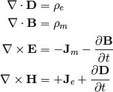
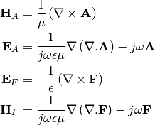
.Vector Potentials and Helmholtz Wave Equations
Assuming the entire system is linear, any source can be separated into
electric and magnetic currents (sources). The vector potentials  and
and  corresponding to these given electric and magnetic currents
 and
and  are given as
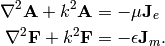
The above equations are derived from the Maxwell’s equations using simple vector identities. Using the Sommerfeld radiation condition, solutions to the above inhomogeneous Hemlholtz equations are given as
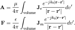
And of course, from the definitions, electric and magnetic fields can be written in terms of the vector potentials as
where  and
and
 . For further details,
please refer to (page.135, [Balanis]).
. For further details,
please refer to (page.135, [Balanis]).
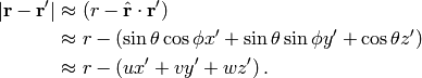
Far-field Approximations
In rectangular co-ordinate system, when  , the term
  can be approximated as
So, far-field vector potentials are given as
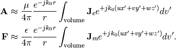
From the above equations, it is evident that  and
and  form Fourier transform pairs.
In comparison to the signal processing terminology,
form Fourier transform pairs.
In comparison to the signal processing terminology,  and
and
 are analogous to time
  and frequency
  , respectively.
Also, far-field electric and magnetic field components can be approximated as (for the
 and
and  components only since
  and
and  )
)
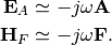
The far-field components  and
and  are related
to the above components as
are related
to the above components as 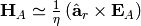 and
and 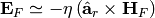 ,
where
,
where  is the free space wave impedance.
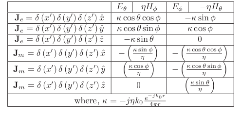
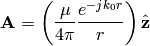
Far-field Green’s Functions of Infinitesimal Dipoles
Now, a simple example will be considered. This example deals with evaluation of
the far-field components corresponding to a infinitesimal electric dipole placed
at the origin and oriented along the  -axis. The corresponding vector potential
is given as
-axis. The corresponding vector potential
is given as
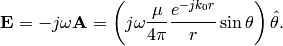
Converting the above equation into spherical co-ordinate system gives
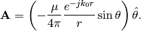
In deriving the above equation, radial component of the vector potential is neglected. Finally, far-field electric field is given as
Similar far-field Green’s functions corresponding to infinitesimal dipoles oriented along various directions are given below.